
Image Enhancement Using Spatial Domain Filtering
Spatial term, refers to pixels which are the smallest element of an im- age. All the changes directly execute these values. Spatial domain could be written in this notation:
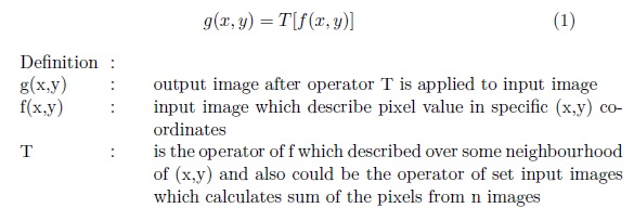
In spatial domain, the simplest form of T is of size 1×1. In this case, g(x,y) depends only the value of f(x,y), and T becomes a gray level. The larger neighbourhoods can also exist. They are known as masks which may vary in the implementation such as filters, kernels, templates or windows [1].
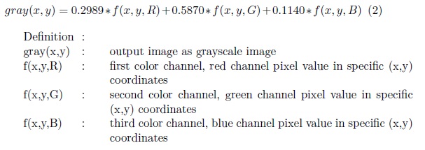
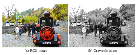
As it is described, grayscale image is used as the input to the algorithm. RGB (Red Green Blue) images are acquired in the acquisition task. These images need to be converted into grayscale images. The purpose of con- verting input image to grayscale aim at minimizing inter-image variances induced by different subject colors. If algorithm is optimized to the spe- cific color, it will be very difficult to work with other colors. Therefore by converting RGB images into grayscale images, it is possible to have one standard format input. The formula of converting RGB to grayscale image as follows:
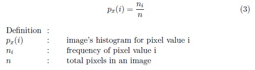
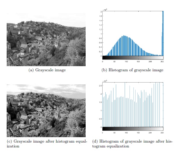
Histogram is also introduced in this spatial domain. Histogram can be described as the image statistics with the gray levels. This calculated statis- tics value, according to the intensity of gray levels that may occurred in specific (x,y) coordinates, can be a useful information in order to do en- hancement.
In this work, histogram equalization is applied in order to adjust the contrast of grayscale image. Uneven illumination may occurred in the ac- quisition task. Therefore by calculating histogram equalization, the image can be enhanced further. The steps which are necessary in order accomplish this task:
- Calculate probability mass function (PMF)
PMF is a frequency of each corresponding pixels.
- Calculate cumulative distributive function (CDF)
CDF is a function that calculates the cumulative sum of all the values that are calculated by PMF.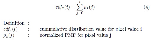
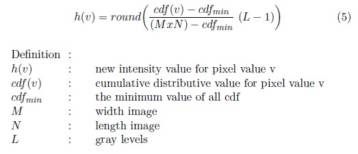
- Calculate CDF according to gray levels
Bibliography
[1] Rafael C. Gonzalez; Richard E. Woods. Digital image processing third edition. Pearson education international, 2008.