Convolutional Neural Network
A convolutional neural network (CNN) is a special kind of neural networks that has been widely applied to a variety of pattern recognition problems, such as computer vision, speech recognition, etc. The CNN was first inspired by [Hubel & Wiesel 62] and continually implemented by many researchers. Some successful implementations of CNN are NeoCognitron [Fukushima 80], LeNet5 [Lecun & Bottou+ 98], HMAX [Serre & Wolf+ 07], AlexNet [Krizhevsky & Sutskever+ 12], GoogLeNet [Szegedy & Liu+ 15], ResNet [He & Zhang+ 15], etc.
Here, we only focus on two dimensional convolutional neural networks. The basic idea of CNN is to build invariance properties into neural networks by creating models that are invariant to certain inputs transformation. This idea originates from a problem that often occurs in the feed forward neural networks, especially multilayer feed forward neural network (MLP). The problem is all MLP layers fully connected to each other. It removes the spatial information of the inputs which are needed for the computational.
Unlike the ordinary neural networks, CNN has a special architecture. The architecture of CNN usually is composed of a convolutional layer and a sub-sampling layer as presented in Figure 1. The convolutional layer implements a convolution operation, and a sub-sampling operation was done in the sub-sampling layer. Here, the sub-sampling is also known as a pooling. CNN is built based on three basic ideas, i.e., local receptive fields, weight sharing, nd pooling.

Local receptive ftelds
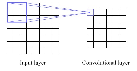
In the feed forward neural network, the input is fully connected to the next hidden node for every neuron. In contrast, the input of CNN only makes the connection within a small region. Each neuron in a hidden layer will be connected to a small field of the previous layer, which is called a local receptive field. For example, if the field has a 3 × 3 area, a neuron of the first convolutional layer is corresponding to 9 pixels of the input layer. Figure 2 illustrates the small coloured box as the local receptive fields, and the coloured lines represent where the neuron is connected to.
Weight Sharing
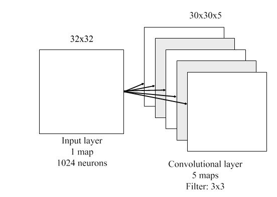
In the convolutional layer, the neurons are organized into multiple parallel hidden layers, which so-called feature maps. Each neuron in a feature map is connected to a local receptive field. For every feature map, all neurons share the same weight parameter that is known as filter or kernel. For instance, Figure 3 describes when an input of 32 × 32 pixels is trained by a convolutional layer with filter 3 × 3 and 5 feature maps.
Pooling
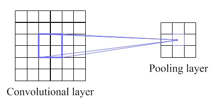
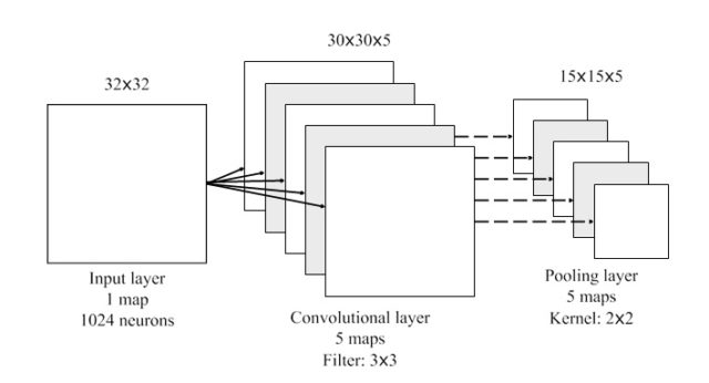
As described earlier, a CNN contains not only convolutional layers, but sometimes also pooling layers. When there is a pooling layer, it is usually used immediately after a convolutional layer. It means the outputs of the convolutional layer are the inputs to the pooling layer of the network. The idea of a pooling layer is to generate translation invariant features by computing statistics of the convolution activations from a small receptive field that corresponds to the feature map. The size of a small receptive field in here depends on the pooling size or kernel pooling. An example of how it works for each feature map is illustrated in Figure 4. If there are more than a single feature map, Figure 5 describes the example of that case.
References
[Fukushima 80] K. Fukushima. Neocognitron: A self-organizing neural network model for a mechanism of pattern recognition unaffected by shift in position. Biological Cybernetics, Vol. 36, No. 4, pp. 193–202, April 1980.
[He & Zhang+ 15] K. He, X. Zhang, S. Ren, J. Sun. Deep Residual Learning for Image Recognition. arXiv:1512.03385 [cs], Vol. 1, Dec. 2015. arXiv: 1512.03385.
[Hubel & Wiesel 62] D. H. Hubel, T. N. Wiesel. Receptive fields, binocular interaction and functional architecture in the cat’s visual cortex. The Journal of Physiology, Vol. 160, No. 1, pp. 106–154.2, Jan. 1962.
[Krizhevsky & Sutskever+ 12] A. Krizhevsky, I. Sutskever, G. E. Hinton. ImageNet Classification with Deep Convolutional Neural Networks. pp. 1106–1114, 2012.
[Lecun & Bottou+ 98] Y. Lecun, L. Bottou, Y. Bengio, P. Haffner. Gradient-based learning applied to document recognition. Proceedings of the IEEE, Vol. 86, No. 11, pp. 2278–2324, Nov. 1998.
[Serre & Wolf+ 07] T. Serre, L. Wolf, S. Bileschi, M. Riesenhuber, T. Poggio. Robust Object Recognition with Cortex-Like Mechanisms. IEEE Transactions on Pattern Analysis and Machine Intelligence , Vol. 29, No. 3, pp. 411–426, March 2007.
[Szegedy & Liu+ 15] C. Szegedy, W. Liu, Y. Jia, P. Sermanet, S. Reed, D. Anguelov, D. Erhan, V. Vanhoucke, A. Rabinovich. Going deeper with convolutions. In 2015 IEEE Conference on Computer Vision and Pattern Recognition (CVPR), pp. 1–9, June 2015.
